This section serves a number of purposes: First, it illustrates the issues that were raised while discussing the parallel implementation of matrix-matrix multiply and its variants. Second, it shows that indeed high performance can be attained using the techniques that underlie PLAPACK. Finally, it demonstrates that high performance can be attained on different architectures without any changes to the infrastructure. However, one should not read too much into the performance graphs: we collected and graphed performance numbers for the part of the infrastructure that was optimized as of the moment that the guide was completed. To see the current performance numbers for a range of algorithms, consult the PLAPACK web page.
All performance numbers center around the implementation
of the most basic case of matrix-matrix multiplication:
![]() . For this case, we will
show the performance of the three variants: panel-panel,
matrix-panel, and panel-matrix.
. For this case, we will
show the performance of the three variants: panel-panel,
matrix-panel, and panel-matrix.
Performance is reported in MFLOPS/sec per node, or millions of floating point operations per second per node. Given that a problem of with dimensions m , n , and k requires time t(m,n,k) (in seconds) to complete, the MFLOPS/sec per node for matrix-matrix multiplication is computed using the formula
![]()
We discuss performance on three current generation
distributed memory parallel computers:
the Intel Paragon with GP nodes (one compute processor
per node),
the Cray T3D, and the IBM SP-2.
In addition, we show performance on the Convex Exemplar S-class system,
in a shared-memory configuration.
In all cases we will report performance per node,
where we use the term node for a compute processor![]() .
All performance is for 64-bit precision (i.e. double precision
real on the Exemplar, the Paragon, and the SP-2, and single precision real on
the T3D).
The peak performance of an individual node limits the
peak performance per node that can be achieved for our
parallel implementations. As of this writing,
the single processor peak performances for 64-bit arithmetic matrix-matrix multiply,
using assembly coded sequential BLAS, are
roughly given by
.
All performance is for 64-bit precision (i.e. double precision
real on the Exemplar, the Paragon, and the SP-2, and single precision real on
the T3D).
The peak performance of an individual node limits the
peak performance per node that can be achieved for our
parallel implementations. As of this writing,
the single processor peak performances for 64-bit arithmetic matrix-matrix multiply,
using assembly coded sequential BLAS, are
roughly given by

The speed and topology of the interconnection network affects how fast peak performance can be approached. Since our infrastructure is far from optimized with regards to communication as of this writing, there is no real need to discuss network speeds other than that both the Intel Paragon and Cray T3D have very fast interconnection networks, while the IBM SP-2 has a noticeably slower network, relative to individual processor speeds. On the Exemplar, we use MPI to communicate between processors, so that it is programmed as if it were a distributed memory architecture.
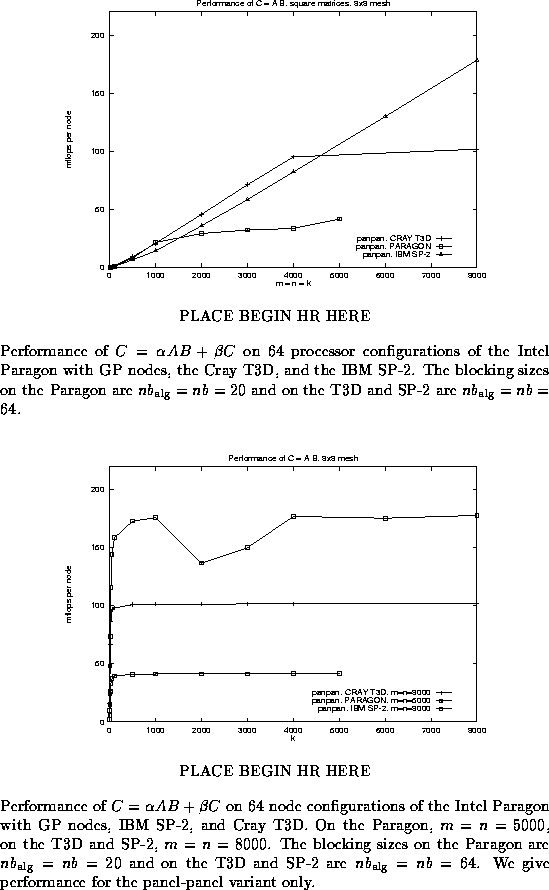
In Figure ![]() , we show the performance
on 64 node configurations of the different architectures.
In that figure, the performance of the panel-panel
variant is reported, with the matrix dimensions chosen so that
all three matrices are square. The algorithmic and distribution
blocking sizes,
, we show the performance
on 64 node configurations of the different architectures.
In that figure, the performance of the panel-panel
variant is reported, with the matrix dimensions chosen so that
all three matrices are square. The algorithmic and distribution
blocking sizes, ![]() and nb
were taken to be equal to each other (
and nb
were taken to be equal to each other ( ![]() ),
but on each architecture they equal the value that appears to
give good performance: on the Paragon
),
but on each architecture they equal the value that appears to
give good performance: on the Paragon ![]() and on the T3D and SP-2
and on the T3D and SP-2 ![]() .
The different curves approach the
peak performance for the given architecture, eventually leveling
off.
.
The different curves approach the
peak performance for the given architecture, eventually leveling
off.
In Figure ![]() , we again report the performance on
the different architectures for the panel-panel variant, with
the same choices for the blocking parameters.
PLACE BEGIN HR HERE
, we again report the performance on
the different architectures for the panel-panel variant, with
the same choices for the blocking parameters.
PLACE BEGIN HR HERE
PLACE END HR HERE
However, this time we fix dimensions m and n to be large, and we vary dimension k . For the panel-panel based implementation, on all architectures high performance is achieved even for small values of k , which verifies that the panel-panel variant is a good choice when k is small. This was predicted when we discussed implementation of the different variants.
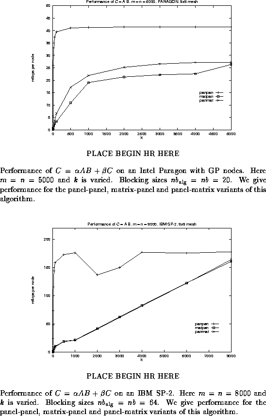
In Figure ![]() , we illustrate the performance
for the different variants on the Intel Paragon, by fixing
dimensions m and n to be large ( m = n = 5000 )
and varying k along the x-axis.
Our previous discussion
predicts that the panel-panel implementation is most natural
for this shape of the matrices, and indeed, that variant outperforms
the other two. One fact worth mentioning is that the matrix-panel
and panel-matrix variants level off at a considerably lower level
of performance. This is due to the fact that the sequential dgemm
implementation performs better for a panel-panel update than
a matrix-panel or panel-matrix multiply when the panel width is 20.
(Notice that this reflects a limitation of the implementation of
the sequential dgemm call. Better performance can be attained
by more careful implementation of that kernel.)
Similar behavior is reported in Figure
, we illustrate the performance
for the different variants on the Intel Paragon, by fixing
dimensions m and n to be large ( m = n = 5000 )
and varying k along the x-axis.
Our previous discussion
predicts that the panel-panel implementation is most natural
for this shape of the matrices, and indeed, that variant outperforms
the other two. One fact worth mentioning is that the matrix-panel
and panel-matrix variants level off at a considerably lower level
of performance. This is due to the fact that the sequential dgemm
implementation performs better for a panel-panel update than
a matrix-panel or panel-matrix multiply when the panel width is 20.
(Notice that this reflects a limitation of the implementation of
the sequential dgemm call. Better performance can be attained
by more careful implementation of that kernel.)
Similar behavior is reported in Figure ![]() for the
IBM SP-2.
PLACE BEGIN HR HERE
for the
IBM SP-2.
PLACE BEGIN HR HERE
PLACE END HR HERE
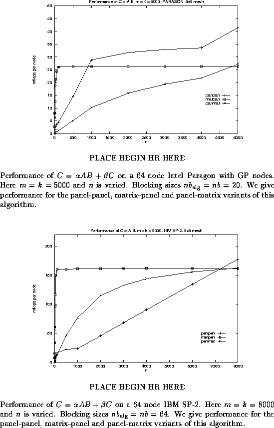
In Figure ![]() , we again illustrate the performance
for the different variants on the Intel Paragon, but this time
dimensions m and k are fixed to be large ( m = k = 5000 )
and n is varied.
Our previous discussion
predicts that the matrix-panel variant is the most natural
for this shape of the matrices, and indeed, that variant initially outperforms
the other two, when n is small.
Since the matrix-panel
and panel-matrix variants level off at a considerably lower level
of performance, due to the sequential dgemm implementation,
eventually the panel-panel variant becomes fastest.
Similar behavior is reported in Figure
, we again illustrate the performance
for the different variants on the Intel Paragon, but this time
dimensions m and k are fixed to be large ( m = k = 5000 )
and n is varied.
Our previous discussion
predicts that the matrix-panel variant is the most natural
for this shape of the matrices, and indeed, that variant initially outperforms
the other two, when n is small.
Since the matrix-panel
and panel-matrix variants level off at a considerably lower level
of performance, due to the sequential dgemm implementation,
eventually the panel-panel variant becomes fastest.
Similar behavior is reported in Figure ![]() for the
IBM SP-2.
PLACE BEGIN HR HERE
for the
IBM SP-2.
PLACE BEGIN HR HERE
PLACE END HR HERE
Notice that showing performance numbers for a single configuration
of an architecture gives no insight into the scalability of the
approach.
As nodes are added, the problem size can grow so that
memory use per node remains constant (after all, as nodes
are added, so is memory). For the matrix-matrix multiply
example, the means that if m = n = k , then the dimensions
can grow with the square-root of the number of nodes.
Generally, dense linear algebra algorithms can be
parallelized so that they are scalable in the following sense:
if the problem size is increased
so that memory use per node is kept constant, then the
efficiency (e.g., MFLOPS/sec per node) will remain
(approximately) constant.
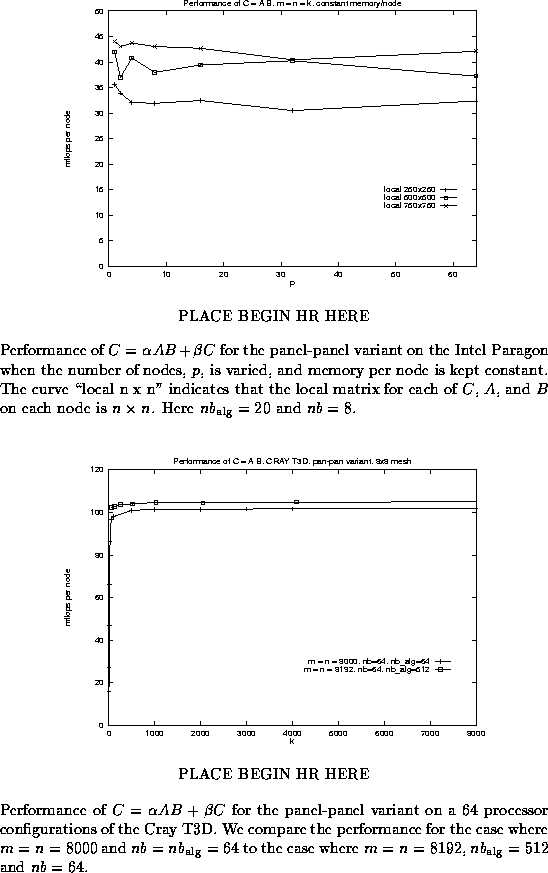
To verify this trend for matrix-matrix multiply,
we report in Figure ![]() the MFLOPS/sec per node on the Intel Paragon when
the number of nodes is varied, and the memory per node
is kept constant. Notice that the performance is only
slightly affected as nodes are added.
the MFLOPS/sec per node on the Intel Paragon when
the number of nodes is varied, and the memory per node
is kept constant. Notice that the performance is only
slightly affected as nodes are added.
In Figure ![]() , we show that by carefully picking
parameters and matrix dimensions, one can further improve performance.
In that figure, we contrast the performance of the panel-panel
variant on a Cray T3D for two slightly different choices:
The first curve shows the exact same data as used in Figure
, we show that by carefully picking
parameters and matrix dimensions, one can further improve performance.
In that figure, we contrast the performance of the panel-panel
variant on a Cray T3D for two slightly different choices:
The first curve shows the exact same data as used in Figure ![]() :
m = n = 8000 and
:
m = n = 8000 and ![]() .
For that curve, no particular care is taken when picking the k
at which the timings were collected.
For the second curve, we increased the problem slightly, to m = n = 8192
(a power of two),
the distribution blocking size was kept at nb = 64 , and
the algorithmic blocking size was increased to
.
For that curve, no particular care is taken when picking the k
at which the timings were collected.
For the second curve, we increased the problem slightly, to m = n = 8192
(a power of two),
the distribution blocking size was kept at nb = 64 , and
the algorithmic blocking size was increased to ![]() .
Also, k was sampled at powers of 2 . Notice that performance improves
slightly.
PLACE BEGIN HR HERE
.
Also, k was sampled at powers of 2 . Notice that performance improves
slightly.
PLACE BEGIN HR HERE
PLACE END HR HERE
In Figure ![]() , we examine the performance of PLAPACK
PLACE BEGIN HR HERE
, we examine the performance of PLAPACK
PLACE BEGIN HR HERE
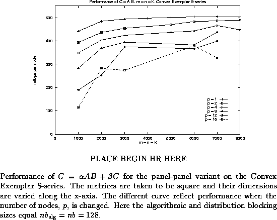
PLACE END HR HERE
on the Convex Exemplar S-series. While all data presented was collected using a single 16 processor shared memory cluster, communication between processors uses MPI, like on a distributed memory architecture. The graph shows performance for square matrices, with the different curves representing different numbers of nodes being used. While trying to meet the deadline for this guide, we did not have time to fully tune PLAPACK for the Exemplar. Nonetheless, very good performance is achieved. It should be noted that for some matrix sizes, performance on the Exemplar was much lower than expected. In order to make the graph less busy, those performance numbers for the Exemplar are not reported. We expect that further experimentation will allow us to more consistently achieve high performance.